AGCN (CVPR 2019, action recognition)

Abstract

• CVPR 2019
• skeleton-based action recognition을 위한 GCN based method
• 2s-AGCN(two-stream adaptive GCN) 제안
• https://github.com/lshiwjx/2s-AGCN

 

 

 

Motivation

ST-GCN에서 처음 GCN을 이용해 skeleton-based action recognition에 활용했다. 하지만 여기에는 세 가지 문제가 있었다:

1. skeleton graph가 heuristic하게 predefine되어 human body의 physical structure만 반영한다.
   (예컨대, "reading"이나 "clapping"에서는 두 손 간의 상호작용이 중요한데, 이는 joint 상에서 멀리 위치하여 dependency가 제대로 반영되기 어렵다)
2. GCN의 structure는 다른 layer가 multilevel semantic information을 담고 있을 때 hierarchical하다. 그러나 ST-GCN에 적용된 graph topology는 모두 동일해서 이런 장점을 갖기 어렵다.
3. fixed graph structure는 different action class에 대해서 optimal하지 않을 수 있다. 

결국 세 개 다 비슷한 이야기이다. 1번하고 3번은 거의 같은 이야기이고, 2번에 대해서 생각해볼 수 있다. 이게 사실 GCN도 message passing하고 같은 형태가 되는데, 모든 node가 다 연결되어 있거나 좀 더 복잡한 형태라면 다른 곳에 왔다가 다시 돌아오는 형태로 multi-hop에 대한 정보를 가질 수 있을 텐데, ST-GCN에서 제안한 graph topology는 거의 단일 경로 형태이다. 따라서 message passing을 해도 한 번에 대부분 양쪽에 위치한 2개의 neighbor에 대해서만 propagation이 된다. 이 점은 좀 더 복합적인 정보를 담기 어렵다고 생각할 수 있다. 

 

 

 

 

Methods

Graph Construction

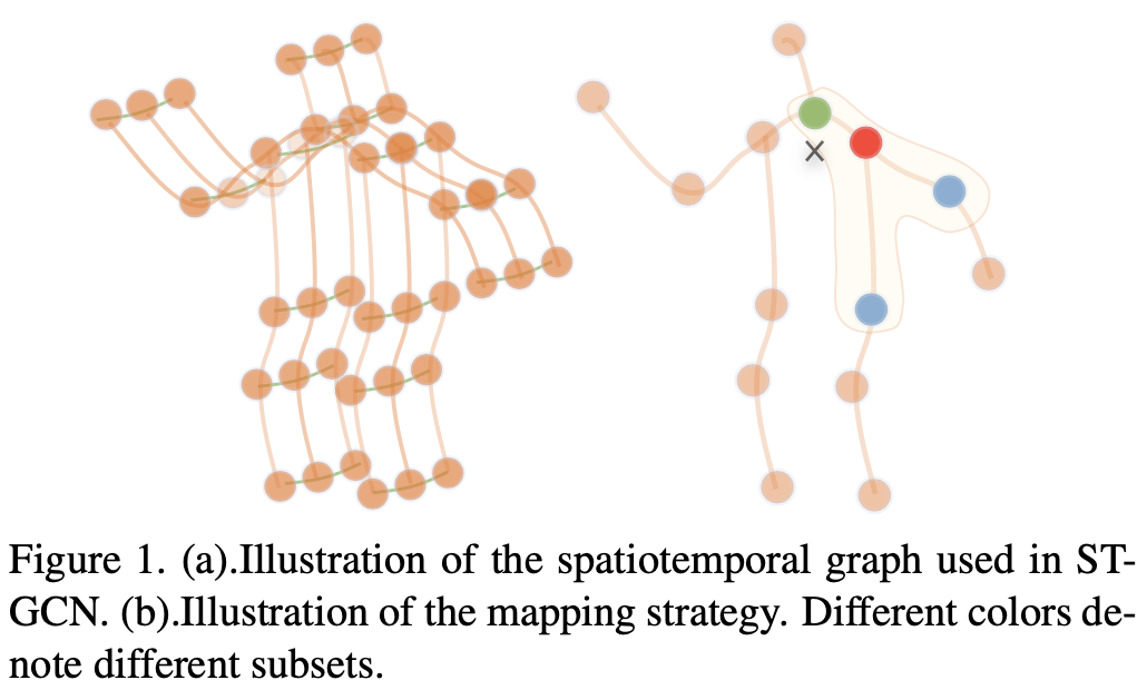
먼저 ST-GCN에서처럼 spatiotemporal graph를 사용한다. Fig. 1(a)에서 주황색으로 표현된 spatial edge와 초록색으로 표현된 temporal edge가 있고, vertex의 attribute는 joint의 coordinate이 사용된다. 

 

 

Graph Convolution

spatial dimension에서 GC operation은 다음과 같이 수행된다: 

 

Equation 1: graph convolution operation in the spatial dimension.

$f$는 feature map, $v$는 vertex, $B_i$는 convolution의 sampling area, $w$는 weighting funciton, $l_i$는 mapping function이다. formulation은 ST-GCN과 비슷하니 이를 참조하면 좋다. 

 

여기서의 결과는 Fig. 1(b)에 나와 있는데, root node, centripetal group, centrifugal group으로 나누어져 있다. 

 

 

ST-GCN Implementation

Equation 2: ST-GCN implementation.

실제 graph는 $ℝ^{C×T×N}$ 크기인데, $A_k= Λ_k^{-1/2}\bar A_k Λ^{-1/2}_k$이다. $M$은 each vertex의 importance를 나타내는 attention map이고, $\odot$은 dot product를 의미한다. 

 

 

 

 

 

 

Adaptive Graph Convolution Layer

 

 

고정된 graph 구조의 문제를 해결하기 위해 제안된 방법으로, 각 layer마다 graph에 residual branch를 추가해서 original model의 stgability를 유지하면서 flexibility를 증가하는 방법이다. 

 

Equation 2.

Eq. 2에서 adjacency matrix가 세 부분으로 나뉜 것을 볼 수 있다:

 

$A_k$는 $N×N$ normalized adjacency matrix A_k를 의미한다. 이는 human body의 physical structure를 represent한다.

 

$B_k$는 $N×N$ adjacency matrix인데, $B_k$의 모든 elements는 parameter이며 training 과정에서 optimize된다. 이외에 다른 constraint는 없다. 이 graph는 각 joint 간의 connection과 connection의 strength를 의미하게 된다. 역할은 $M_k$와 비슷하지만 원래 $0$이었던 connection을 create할 수 없었다는 dot product의 문제를 해결한 좀 더 flexible한 방식이다.

 

$C_k$는 각 sample에 대해 unique graph를 learn하는 data-dependent graph이다.

Equation 4.

이는 embedded Gaussian function을 이용하여 두 vertex의 similarity를 계산한다. Eq. 4를 보면 $v_i$와 $v_j$의 feature에 대해서 embedding function $θ,φ$를 이용해서 $ℝ^{C_{in}×T×N}→ℝ^{C_e×T×N}$ mapping을 한다. embedding function은 1×1 convolution이다. 

 

그 후 두 feature map은 $N×C_eT$와 $C_eT×N$ 크기 matrix로 reshape된 후 $N×N$ similarity matrix $C_k$를 계산한다. 이 값은 $[0,1]$으로 normalize되는데, 이를 종합하면 다음과 같다.

 

 

$C_k$는 original $A,B$에 단순히 더해지는 방식으로 사용된다. 이는 original model의 performance를 preserve하면서 flexibility를 향상하는 역할을 한다. 

 

여기에 residual 값에 1×1 convolution을 한 뒤 더해주면 Fig. 2의 전체 flow가 된다. 

 

 

 

Adaptive Graph Convolutional Block

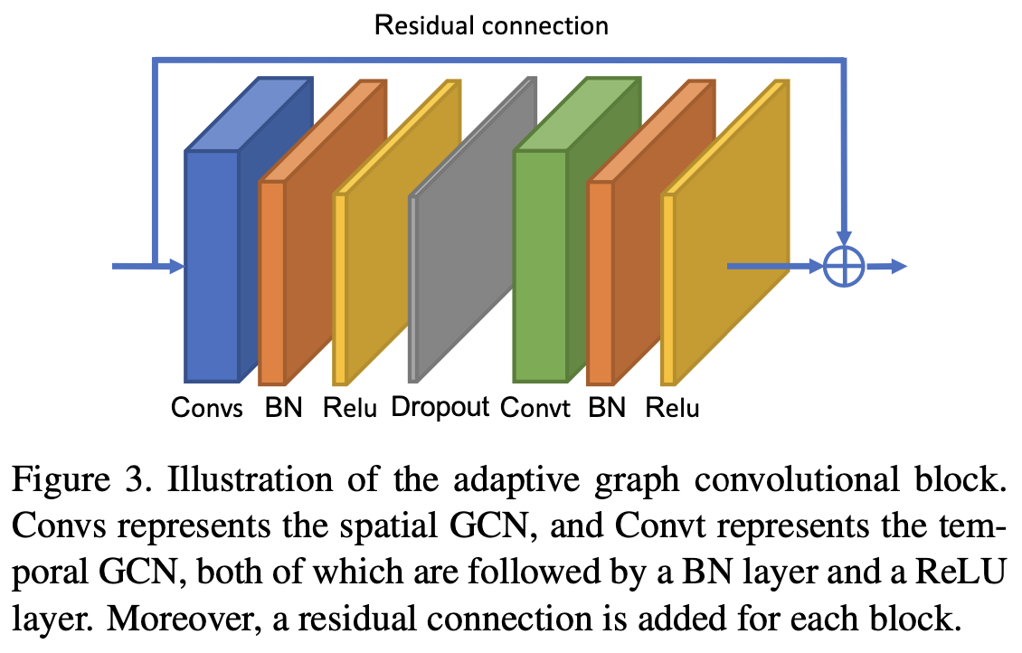
ST-GCN처럼 $K_t ×1$ convolution을 수행한다. 먼저 spatial하게 수행하고(Convs) 그 후 temporal하게 수행한다(Convt).

 

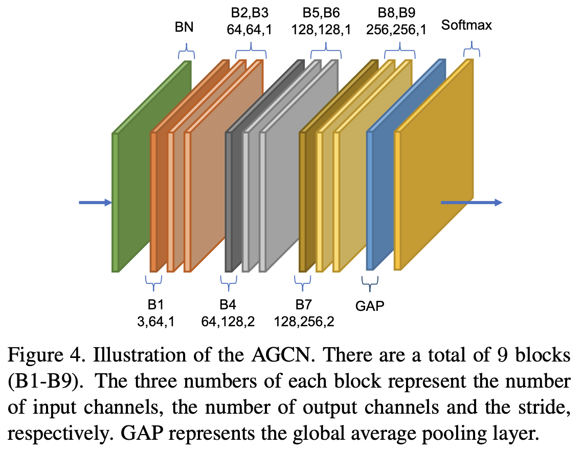
Fig. 4에서 이런 block들을 쌓아서 adaptive convolutional neural network(AGCN)을 구성한 것을 볼 수 있다. 마지막에 global average pooling으로 graph를 pooling한다. 

 

 

 

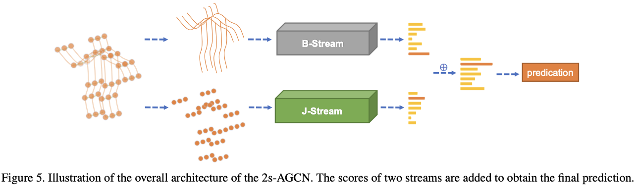
Two-stream Networks

또한, AGCN에서는 특이하게 bone information도 활용한다. bone이라고 하면 두 인접한 joint끼리 연결성을 vector로 표현한 것이다. 즉, source joint $v_1 = (x_1,y_1,z_1)$와 target joint $v_2=(x_2,y_2,z_2)$를 연결하는 bone vector는 $e_{v_1,v_2}=(x_2-x_1,y_2-y_1,z_2-z_1)$이 된다. 

 

각각의 bone은 unique한 target joint를 갖게 된다. central joint는 어떤 bone도 assign되지 않으므로 bone의 개수는 joint의 개수보다 하나 적다. cycle이 없는 tree 구조에서 선분의 개수는 점의 개수보다 하나 적은 것과 마찬가지이다. 

 

network를 간단하게 하려면 joint와 개수가 같아야 하므로, central joint에는 value가 0인 empty bone을 설정하였다. 이 방식으로 joint를 계산하는 J-stream과 bone을 계산하는 B-stream을 각각 구성하였다. 마지막에 두 stream의 score가 합해 fused score를 얻은 뒤 action label을 predict한다.

 

 

두 stream의 유효성은 ablation study에서 확인된다. 

 

 

 

Experiments

Ablation Study

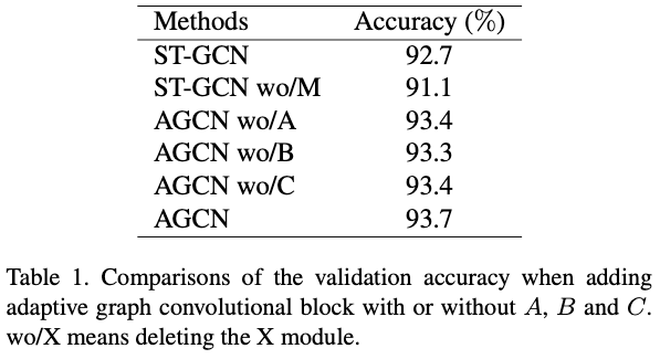
• Adaptive graph convolutional block

 

• Visualization of the learned graphs 

 

 

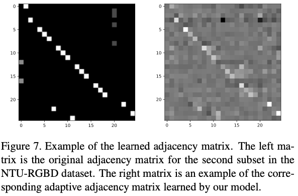
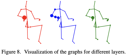
Fig. 8은 25번째 joint와 각 joint의 connection의 강도를 점의 크기로 표현했다. 왼쪽부터 3th, 5th, 7th layer의 값이다. 25번째 joint가 무엇인지 정확히 알려주지 않았지만, 오른쪽 팔 근처의 joint로 생각된다. 

 

초반 layer의 경우 adjacent한 joint에 strong connection을 가지고 있지만, 뒤쪽 layer는 body의 physical structure를 넘어서 다른 joint에 strong connection을 가진다. 이는 graph가 점점 final classification task에 맞는 형태를 갖게 됨을 의미한다고 해석한다. 

 

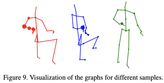
Fig. 9는 같은 layer의 다른 sample에 대한 결과이다. 서로 다른 부분에 집중됨이 보인다. 

 

• Two-stream framework

Tab. 2는 bone이 포함된 경우 성능 향상됨을 보인다.

 

다만 내 생각에는 굳이 bone graph가 필요할 것 같지 않다. 그냥 좌표 값 간 차이라는 feature는 network 안에서도 학습이 가능하니까 같은 데이터를 두 번 넣어준 느낌이다. 2s-AGCN을 넣어서 성능이 향상된 건 자세한 실험 세팅은 알 수 없지만 아마 network capacity 차이 때문 아니었을까.

 

 

 

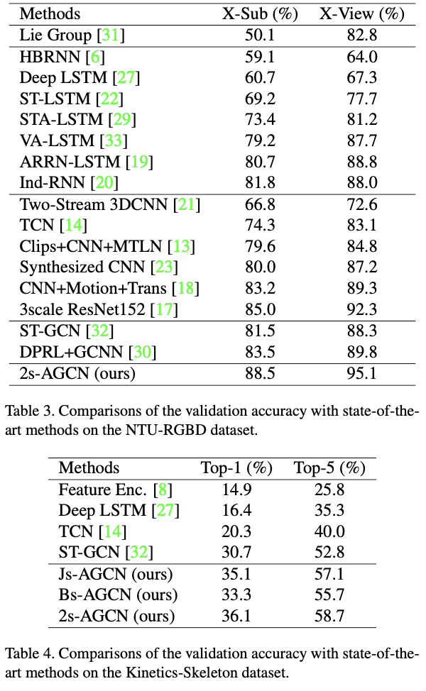
Results

 

 

 

 

 

Discussion

 

 

---

References

[1] Shi, L., Zhang, Y., Cheng, J., & Lu, H. (2019). Two-stream adaptive graph convolutional networks for skeleton-based action recognition. In Proceedings of the IEEE/CVF conference on computer vision and pattern recognition (pp. 12026-12035).

Footnotes