Abstract
- ICCV 2023
- 3D human pose estimation in monocular video
- GLA-GCN 제안, graph representation으로 joint의 spatiotemporal structure model
- global representation과 local representation을 모두 활용하여 3D pose estimation
- https://github.com/bruceyo/GLA-GCN
Prerequisite
- ST-GCN[2] (https://jordano-jackson.tistory.com/137 참조)
- AGCN[3] (https://jordano-jackson.tistory.com/138 참조)
Motivation
기존의 방법론은 크게 TCN(Temporal Convolutional Network), GCN, Transformer based model로 나눌 수 있다. TCN과 Transformer based approach는 flattened sequence 형태로 입력을 받으므로 pose structure에 대한 intuitive design을 만들기 어렵다. 따라서 GCN based approach를 시도한다.
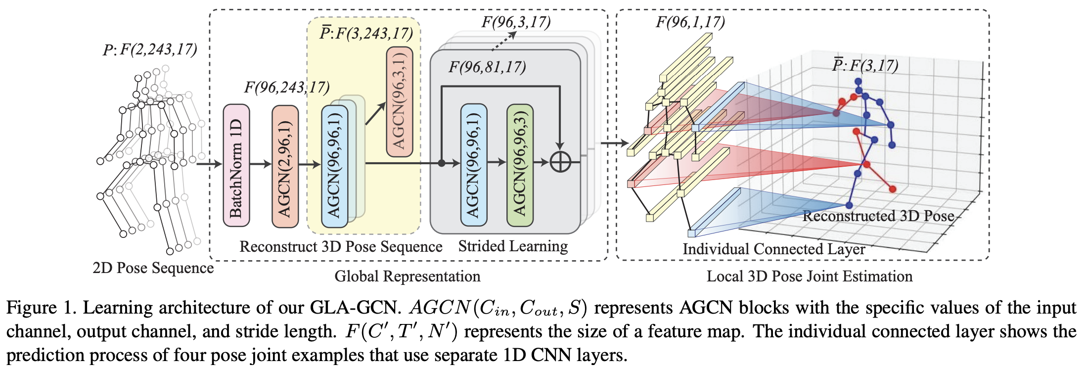
GLA-GCN은 global representation과 local 3D pose estimation의 두 개의 module로 구성되어 있다. global representation에서는 AGCN을 사용해서 2D sequence에서 3D representation을 reconstruct한다.
local 3D pose joint estimation에서는 global representation을 shrink한 뒤 이를 이용해 3D pose joint를 estimate한다.
Methods
task의 목적은 video에서 2d로 주어진 pose sequence $P = \{p_{t,i} \in ℝ^2 | t= 1, \dots, T; i= 1, \dots, N\}$에서 3D pose joint의 coordinate $\bar P = \{ \bar p_i \in ℝ^3|i=1,\dots, N\}$를 reconstruct하는 것이다. ($T$: the number of pose frames, $N$: the number of pose joints)
Global Representation
- Adaptive Graph Convolutional Network
AGCN 게시글에 정리해 놓았으므로 생략한다.
- Reconstruct 3D pose sequence
AGCN block을 train하기 위해서 2D sequence에서 3D sequence를 estimate하여 supervised manner로 학습한다. 이는 Fig. 1의 Reconstruct 3D Pose Sequence 부분을 확인하면 된다.
2D pose sequence는 $F(2,T,N)$ 사이즈이다. Human3.6M dataset에서는 $T=243, N=17$이다. 여기에 처음 $AGCN(2,96,1)$을 적용해서 feature channel을 96D으로 만든다.
이 output은 $F(96, 243, 17)$이 되고, $AGCN(96,96,1)$ layer를 몇 번 더 쌓는다. 마지막에 $AGCN(96,3,1)$으로 3d pose를 96D joint representation을 이용해 estimate한다. ($AGCN(C_{in}, C_{out}, S)$의 parameter는 input channel $C_{in}$, output channel $C_{out}$, temporal convolution의 stride $S$이다.)
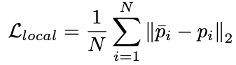
최종적으로 $\dddot p_{t,i}\in ℝ^3$이 $i$th joint의 time $t$에서의 3D position이라고 하면, 3D pose sequence의 loss는 Eq. 4와 같이 계산된다:

- Strided learning architecture
strided AGCN module은 Fig. 1의 gray block 부분이다. 해당 module은 TCN-based approach에서 motivate된 것으로, strided convolution을 이용하여 긴 time sequence를 줄이고 $t$ time 근처의 temporal information을 aggregate한다.
각 strided AGCN module은 두 개의 consecutive한 AGCN block과 residual connection으로 연결되어 있다. 이 중 두 번째 AGCN은 stride가 3으로 한 번에 temporal dimension이 3씩 shrink한다. 이를 계속 반복하여 feature size가 $96×1×17$까지 shrink시킨다.
이 방법으로 temporal dimension의 pose sequence가 aggregate되어 centric timestep의 3D pose를 estimate하는데 활용된다.
Local 3D Pose Joint Estimation
strided convolution을 이용해 얻은 $F(96, 1, 17)$ feature map을 이용해서 3D position을 estimate한다.
- Individually connected layers
이전 method에서는 global skeleton representation을 이용하여 모든 single joint를 estimate한다. 그러나 전체 feature map을 이용해서 모든 joint를 estimate하므로 joint 간 correspondance를 고려하지 못한다는 문제가 있음을 지적한다.
따라서 여기서는 aggregated global representation의 corresponding joint node feature $F(96,1,1)$만을 이용하여 corresponding individual joint를 따로 estimate한다. 즉,

Eq. 5에서 $\dot p_i$는 estimated 3D joint $i$의 position, $v_i$는 joint node $i$의 flattened feature $F(96, 1, i)$, $W_i\in ℝ^{96×3}$와 $b_i \in ℝ^{1×3}$은 parameter이다.
이때 weight와 bias는 share되지 않으므로, 각각은 따로 계산할 수 있다. 그러나 이 형태는 2d-to-3d lifting 과정에서의 shared rule을 ignore하여 joint-speicifc distribution을 overfitting하는 경향이 있어서 individually connected layer를 만든 후(Eq. 6) convex combination을 이용하였다. (Eq. 7)


이는 실제로는 1D CNN으로 구현되었다. 결과적으로 local joint의 loss는 다음과 같이 정의된다:
training 과정은 두 stage로 나뉘는데, $L_{global}+L_{local}$을 먼저 minimize하고, second stage에서 $L_{local}$을 minimize하여 3D estimation performance를 improve한다.
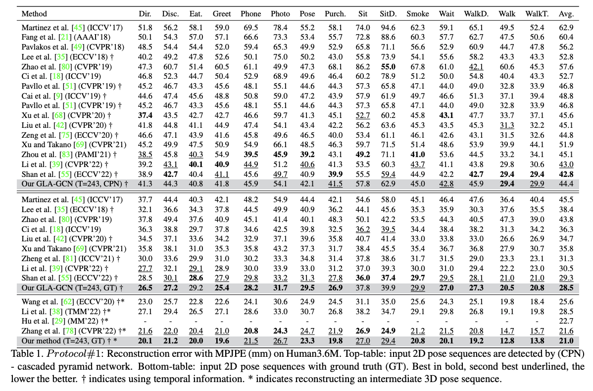
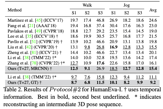
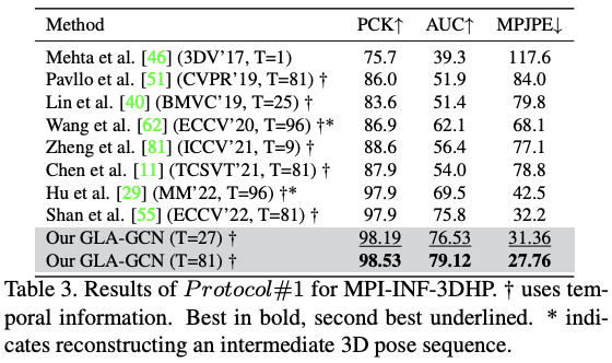
Results
Discussion
References
[1] Yu, B. X. B., Zhang, Z., Liu, Y., Zhong, S., Liu, Y., & Chen, C. W. (2023). GLA-GCN: Global-local adaptive graph convolutional network for 3D human pose estimation from monocular video. In Proceedings of the IEEE/CVF International Conference on Computer Vision (ICCV) (pp. 8818-8829).
[2] Ruoyu Li, Sheng Wang, Feiyun Zhu, and Junzhou Huang. Adaptive graph convolutional neural networks. In Proceedings of the AAAI Conference on Artificial Intelligence, volume 32, 2018.
[3] Lei Shi, Yifan Zhang, Jian Cheng, and Hanqing Lu. Two-stream adaptive graph convolutional networks for skeleton- based action recognition. In Proceedings of the IEEE Conference on Computer Vision and Pattern Recognition, pages 12026–12035, 2019.
[4] Sijie Yan, Yuanjun Xiong, and Dahua Lin. Spatial temporal graph convolutional networks for skeleton-based action recognition. In 32nd AAAI conference on artificial intelligence, 2018.
Footnotes
'DL·ML > Paper' 카테고리의 다른 글
| MViT v1 (ICCV 2021, Video Recognition) (0) | 2024.05.18 |
|---|---|
| U-Net (0) | 2024.04.15 |
| AGCN (CVPR 2019, action recognition) (0) | 2024.04.02 |
| ST-GCN (AAAI 2018, human action recognition) (0) | 2024.04.01 |
| CLIPSelf (ICLR 2024 spotlight, open-vocabulary dense prediction) (0) | 2024.03.29 |