[GNN] GCN을 이용한 Image Captioning

 

 

 

https://arxiv.org/abs/1809.07041

Exploring Visual Relationship for Image Captioning

Abstract

GCN과 LSTM을 결합한 architecture를 이용하여 semantic and spatial object relationship을 image encoder에 반영한다. 

 

Introduction

CNN이나 RNN 기반 image encoding 방법은 image 안의 object 간 relationship을 반영하지 못한다는 한계가 있다. 이 paper에서는 어떻게 image 내의 object 간 inherent relationship을 반영하여 holistical한 방식으로 image를 해석할 수있는지에 대해 다룬다. 

 

여기서 다루는 connection은 semantic connection과 spatial connection으로 나눌 수 있다. 각 graph는 detected region을 vertex로 하고 relationship을 edge로 한 directed graph로 구성된다. GCN은 그 이후 graph representation을 enrich하기 위해 사용된다.

 

Figure 1

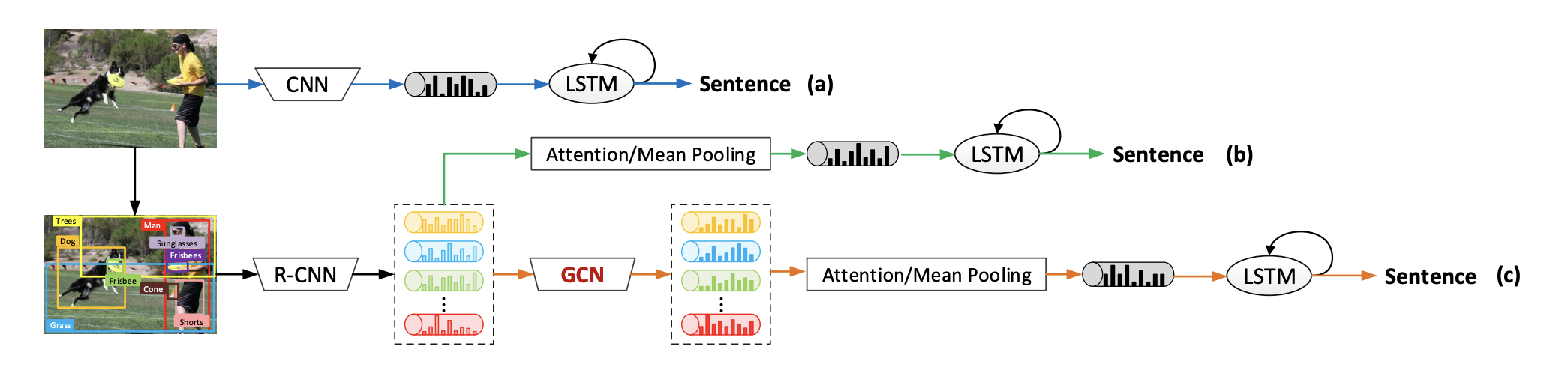
전체적인 flow는 아래 줄과 같다. 이미지에서 R-CNN을 통해 region proposal을 받고, region으로 graph를 만든다. GCN을 돌린 후 attention LSTM decoder로 sentence를 만든다. 

---

Image Captioning by Exploring Visual Relationship

Figure 2

위에서 설명한 아키텍처를 그림으로 나타내면 Figure 2와 같다. R-CNN으로 image region을 얻어서, 두 종류의 그래프로 encoding하고, LSTM attention mechanism으로 decode한다. 

 

또한 sentence generation problem의 loss는 다음과 같은데, 

 

$$ E(V,G,S) = -\log Pr(S|V,G)$$

 

$V$는 regions of objects, G는 constructed rleation graph, S는 sentence이다. 이런 negative log likelihood는 cross entropy loss로 계산되는 경우가 많다. 이 경우 training과 inference 간 차이가 발생하므로 LSTM을 expected sentence-level reward loss로 직접 optimize한다.

 

=> 추가 설명 필요

 

Semantic Object Relationship

여기서는 일반적인 semantic relation이 $<subject-predicate-object>$의 관계로 나타나는 점에서 착안했다. 즉, 두 noun 간 predicate로 연결되는 것이 의미론적 연결의 일반적인 형태이므로, simple deep classification model을 이용해서 $v_i$와 $v_j$ 사이의 semantic relation을 예측했다. 이것은 union bounding box를 이용하여 만들었다.

 

Figure 3

Figure 3은 semantic relation detection framework를 보여준다. 보면 붉은색 region과 초록색 region이 $v_i$와 $v_j$ 로 embedding되는데, 이에 더하여 두 bounding box를 포함하는 union bounding box인 노란색 region도 $v_{ij}$로 embedding 된다.  그 후 featrue들은 concate하고, softmax layer를 거쳐 두 object의 관계를 classify하게 된다. 

 

그럼 이미지에 $K$개의 region of object가 있다고 했을 때 $K(K-1)$개의 관계 pair가 나올 수 있다. 이떄 classification에서 non-relation class를 포함한 $N_{sem}+1$ class 중 하나로 classify해서 non-relation class의 probability가 0.5보다 작을 경우에만 edge를 만든다. edge의 label은 maximum probability인 class가 된다. 

 

 

Spatial Object Relationship

Spatial object relationship은 두 region 간 관계를 object j의 object i에 대한 관계 $<object_i-object_j>$ pair로 본다. 그리고 Figure 4에 따라서 총 11개의 class로 나눈다.

Figure 4

파란색 bounding box가 j이고 붉은색이 i이다. class 1, 2, 3은 special case이다. 세 class에 해당하지 않을 경우 relative distance/diagonal length ratio $\phi_{ij}$를 계산해서 0.5 미만일 경우 4-11은 각도에 따른 클래스를 결정한다. 만약 IoU가 0.5보다 작고 ratio $\phi_{ij}$도 0.5보다 클 경우 spatial한 관계가 약하다고 보고 edge를 만들지 않는다. 

 

이 graph는 every object에 대해 edge를 만든다. 그리고 각각 edge에 대해 위의 관계에 따라 class label이 붙는다. 

 

 

GCN based Image Encoder

original GCN은 undirected graph에서 동작한다. 

 

$$v_i^{(1)} = \rho \left(\sum _{v_j \in N(v_i)} Wv_j +b\right )$$

 

여기에 directed graph의 방향에 따라 사용하는 weight가 다르고, edge의 label에 따라서 사용하는 bias가 달라야 하므로 

 

$$ v_i^{(1)} = \rho \left(\sum _{v_j \in N(v_i)} W_{\text{dir}(v_i,v_j)}v_j +b_{\text{lab}(v_i,v_j)}\right ) $$

 

형태로 사용한다.

 

여기에 추가로 edge-wise gate unit $g$를 도입하는데, 이는 GCN이 좀 더 중요한 edge에 집중하도록 하는 상수이다. 따라서 

 

$$v_i^{(1)} = \rho \left(\sum _{v_j \in N(v_i)} g_{v_i,v_j}\left(W_{\text{dir}(v_i,v_j)}v_j +b_{\text{lab}(v_i,v_j)}\right)\right )$$

$$g_{v_i,v_j}=\sigma\left (\tilde W_{\text{dir}(v_i,v_j)}v_j +\tilde b_{\text{lab}(v_i,v_j)} \right)$$

 

로 사용한다. 

 

Q1. 그럼 vertex(object)의 feature는 뭘로 정의하냐?

 

Q2. edge의 클래스는 어디에서 반영한다는거냐?

-> (vi, vj)의 레이블에 따라 다른 bias 값을 더해준다. 근데? 어차피 bias값은 랜덤 아닌가? 

 

Attention LSTM Sentence Decoder 

LSTM decoder는 위와 같이 구성된다. 

• Attention LSTM decoder collects word, previous state,
  image feature and concats them :
  $$ h_t^1 =\left [ h^2_{t-1}, W_sw_t, \overline v \right ] $$
   
• Normalized attention distribution over all the relation-
  aware region-level feature is generated as :
  $$a_{t,i} = W_a \left[\tanh \left (W_fv_i^{(1)} + W_hh_t^1\right)\right], \lambda_t =softmax(a_t)$$
   
• Second-layer LSTM unit is calculated as :
  $$ h^2_t = f_2\left( \left[ \hat v_t, h^1_t  \right]\right) $$
   

 

 

---

References

 

Footnotes